A work colleague asked me to do a “Mate’s rate” job for his team yesterday.
They had a MS Word document with a huge table in it that they needed to convert to Excel to load into an application.
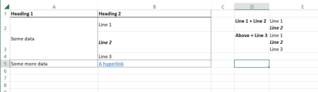
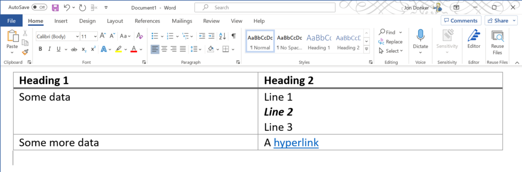
Paraphrased it looked like this:
My first thought was to copy this table out and paste it into excel to see how it looks:
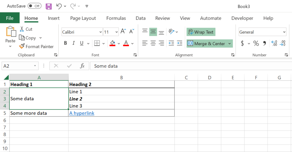
Two problems:
- The cell “Some data” is merged across three rows
- Line 1, Line 2, Line 3 are now split across three rows instead of being in the one cell
I wrote a macro to split out the merge cells; but when it came to combining cells for Line 1, Line 2 and Line 3 I ran into a problem.
None of the usual commands and from my quick google searching could combine the cells and retained the formatting.
So commands like:
=CONCAT(B2:B4)

=B2 & B3 & B4
Would not retain the formatting; let alone add in line feed characters to make it a multiline cell
I’m sure there is a better way – but strapped for time I programmed the following subroutine in VBA
Public Sub combineCells(cell1 As Range, cell2 As Range, output As Range)
    Dim formatIndex As Long
    Dim formatOffset As Long
    Dim hyperlink1 As String
    Dim hyperlink2 As String

    hyperlink1 = ""
    hyperlink2 = ""

    ' Check if the cell has a hyperlin; but don't have a text version of the hyperlink in the Value 2
    If cell1.Hyperlinks.Count <> 0 And InStr(cell1.Value2, "https:") < 1 Then
        hyperlink1 = " [" & cell1.Hyperlinks(1).Address & "]"
    End If

    If cell2.Hyperlinks.Count <> 0 And InStr(cell2.Value2, "https:") < 1 Then
        hyperlink2 = " [" & cell2.Hyperlinks(1).Address & "]"
    End If


    ' Handling if the first cell is blank.  If so we don't want a LF at the top of the cell
    If Trim(cell1.Value2) <> "" Then
        output.Value2 = cell1.Value2 & hyperlink1 & vbLf & cell2.Value2 & hyperlink2
        formatOffset = Len(cell1.Value2) + Len(hyperlink1) + 1
    Else
        output.Value2 = cell2.Value2 & hyperlink2
        formatOffset = Len(cell1.Value2)
    End If


    ' Copies the formatting from cell1 to the final cell
    ' You can add more options to transfer over different formatting
    For formatIndex = 1 To Len(cell1.Value2)
        output.Characters(formatIndex, 1).Font.Bold = cell1.Characters(formatIndex, 1).Font.Bold
        output.Characters(formatIndex, 1).Font.Italic = cell1.Characters(formatIndex, 1).Font.Italic
        'output.Characters(formatIndex, 1).Font.Underline = cell1.Characters(formatIndex, 1).Font.Underline
    Next


    ' Copies the formatting from cell2 to the final cell
    For formatIndex = 1 To Len(cell2.Value2)
        output.Characters(formatIndex + formatOffset, 1).Font.Bold = cell2.Characters(formatIndex, 1).Font.Bold
        output.Characters(formatIndex + formatOffset, 1).Font.Italic = cell2.Characters(formatIndex, 1).Font.Italic
        'output.Characters(formatIndex + formatOffset, 1).Font.Underline = cell2.Characters(formatIndex, 1).Font.Underline
    Next

End Sub
Oh boy it runs slow – to combine a couple of thousands cells took half an hour and I had the typical worries that Excel crashed because everything was locked up.
But it worked for the quick task that I was doing